OFDM
– Multi Carrier Modulation
– Fourier Transformation
– Fast Fourier Transformation (FFT)
Direct Conversion Receiver
Smartphone Technologies
– Multi Touch Display
– Gesture Control
– Distance Sensors

Advanced Technologies for Mobile Broadband and Smartphones

Orthogonal Frequency Division Multiplexing

All previous types of modulation that have been discussed so far use a single carrier frequency and a modulation. The different properties of the transmission differed primarily in the bandwidth used.

However, as early as the 1950s, people were thinking about using several carriers at the same time to transmit information. This was called Multi Carrier Modulation (MCM).

Multi Carrier Modulation

The idea behind MCM is that it is possible to run a lot of narrow-band transmissions in parallel. The narrower the bandwidth of the transmissions, the longer the digital symbols that are sent. This has the advantage that there are only minor problems with intersymbol interference. With broadband signals like W-CDMA, you have extremely short symbols and have to build complex receivers in order to eliminate the effects of multipath propagation. The disadvantage of the low transmission rate of the individual carriers can be compensated for by placing as many carriers as possible in parallel next to each other.

There was another significant effect with MCM that was first described by a Bell Labs engineer named R.W.Chang in 1966.

A carrier signal has a fixed frequency. If the signal is not modulated, the spectrum at the corresponding frequency is a line and is infinitely narrow. If the signal is modulated, the line widens. Depending on the modulation, the signal becomes more or less broad. If we modulate the signal with a square wave function of length T, it is relatively easy to calculate what the spectrum will look like. It has a so-called Sinc function, i.e. Sin(x)/x.

This function is 1 at carrier frequency and then drops to zero at a distance of 1/T. With multiples of 1/T it goes back to zero as you can see in the following figure. You can therefore place a second carrier with a 1/T higher frequency next to the first carrier. This falls exactly to the zero point of the neighboring frequency. The two neighboring beams therefore do not interfere with each other. Since they do not interfere with each other and are “independent” of each other, they are also called orthogonal to each other.

R.W. Chang discovered and patented a process in which, as described above, many narrowband carriers are placed orthogonally from one another, thus representing a new type of modulation that he called Orthogonal Frequency Division Multiplexing (OFDM).

However, the realization of OFDM was practically impossible. With the technology of the time, it would have been necessary to build a transmitter for each carrier and to precisely compare and synchronize it with the neighboring transmitters. This reached its limits after just a few carriers. A solution was proposed in 1971, namely not to generate an OFDM signal from individual carriers but to synthesize the OFDM signal and then radiate it via a single carrier. This required an algorithm called the Fourier Transformation.

Fourier Transformation

Jean Baptiste Joseph Fourier was a French mathematician and physicist at the time of the French Revolution. In a mathematical paper he showed that a periodic signal can be broken down into a series of sine and cosine functions. For example, a square wave signal can be represented by adding sine functions. The first sine has the same frequency as the square wave function. The next sine has three times the frequency and a smaller amplitude, the next sine has five times the frequency and again a smaller amplitude, and so on. In fact, a square wave signal also produces a line spectrum with the fundamental frequency of the square wave signal and further lines decreasing in amplitude at three, five and seven times the frequency.

The Fourier series connect the time domain with the frequency domain.

An extension of the Fourier series is the Fourier transform. It also applies to non-periodic functions. It says that any (time-limited) signal can be generated using sine and cosine functions. The Fourier transform consists of an integral over the frequency of a complex signal. The only important thing at this point is that the Fourier transformation is able to convert any time signal into a complex frequency signal without any information being lost. A complex frequency signal in this case means either a pair of cosine and sine at a specific frequency or an amplitude and phase at a specific frequency. We had already learned from modulation technology that every frequency signal can be represented by cosines and sines.

For a long time, however, the Fourier transform was of more mathematical interest. Only for a few functions the Fourier Transformation could be solved. This changed with computers, which made it possible to calculate integrals numerically. If the time signal is represented in sample values via pulse code modulations, the integral becomes a sum. In order to calculate the associated 1024 complex frequency values from a sequence of 1024 sample values, 1024 x 1024 complex multiplications and additions are necessary. This is a significant amount of computing power even for computers from the 1960s.

Nevertheless, the Discrete Fourier Transform (DFT) became an enormously helpful and useful tool for science, especially for acoustics. Spectral analysis of sounds was extremely difficult and time-consuming, especially when they were not periodic. With the DFT it was possible to spectrally analyze any acoustic signal, which brought great progress for research.

Fast Fourier Transformation (FFT)

Many researchers where working on and with the DFT in the 1960s. Two researchers named James Cooley and John W. Tukey found the computational effort of DFT too high. They wanted a faster signal analysis for their application. As a matter of fact, they discovered that the DFT could be simplified dramatically. They took advantage of the fact that certain calculation steps were repeated and did not actually have to be calculated twice. The new algorithm they developed for calculating the DFT was called Fast Fourier Transform (FFT). This algorithm allowed the Fourier transform to become a more integral and efficient part of digital signal processing and could be used in more and more applications.

It later turned out that the algorithm found was a “rediscovery”. Carl Friedrich Gauß had already developed this algorithm in 1806 to efficiently calculate the trajectory of asteroids.

In 1971, two researchers again from Bell Laboratories made an innovative proposal for OFDM, which then prevailed. They suggested using an FFT or the inverse FFT (iFFT) to generate OFDM signals. In this case all subchannels are generated in the frequency domain. Afterwards an iFFT (inverse FFT) can be used to generate a complex time signal, which can be modulated and transmitted onto a single carrier frequency.

The following figures show a transmitter and a receiver. A data stream is first converted into parallel streams, which are distributed across different frequencies or subbands. Here the data is converted into symbols which correspond to complex amplitudes. An inverse FFT generates a complex time signal which is then modulated to a carrier frequency.

At the receiver, the complex time signal (i and q signal) is brought into the frequency range using Fourier transformation. There the symbol is detected and then converted back into a data stream.

An OFDM process has been known since 1971. However, it took another twenty years until microelectronics was so advanced that an FFT could be calculated fast enough for a transmitter or receiver to work in real time.

The first application of OFDM in a standardized system was Digital Audio Broadcasting (DAB). DAB has been developed in Europe since the late 1980s as the successor to FM Radio. The standard was published in 1995. Up to 1536 subcarriers are used and a bit rate of 2304 kbit/s is achieved. As we have already discussed, MP2 was used to encode the audio signal. However, it took a very long time for DAB to become established. The first DAB transmitters became established towards the end of the noughties and receivers were gradually purchased. Predictions that DAB would quickly replace FM did not come true.

Direct Conversion Receiver

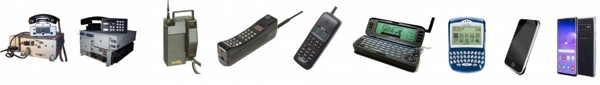
From 2000 onwards, mobile phones stopped getting smaller. Nevertheless, there was pressure to shrink electronics ever smaller. New chips were added to feature phones and smartphones and the display and battery also became increasingly larger. This left less and less room for classic reception electronics. One area for higher integration was the receiver.

Since the beginning, a super heterodyne receiver has been used to receive radio signals. This initially didn’t change for mobile communications either. The following figure shows a typical receiver used in the early days of GSM.

It requires two oscillators. VCO1 to select the channel and a second oscillator VCO2 to mix down to baseband. There is an RF filter to filter the frequency band and an IF filter to eliminate the neighboring bands. Finally, in the baseband, low-band filters for the final suppression of higher frequencies in preparation for the analog-to-digital conversion. Also two amplifiers for the HF and IF domain are required.

The question was raised early on as to whether it was possible to save the intermediate frequency and mix it down directly from the carrier frequency to the baseband. Such a receiver architecture is called direct conversion. Often this architecture is called Zero IF, i.e. “no intermediate frequency”. However, there are major challenges in terms of circuit technology with Zero IF.

With Zero IF, the mixing frequency is exactly the carrier frequency of the transmitter. It must be precisely synchronized, not only in frequency but also in phase. So, a coupling of the carrier with the internal oscillator is required. This can be achieved using phased locked loop techniques that we have already discussed.

The second challenge is that the internal oscillator frequency could „leak“ into the receive path. It is exactly on the reception frequency. In this case it would immediately mask a low input signal and it would no longer be detectable.

Thirdly, it must be prevented that signals that are in the image frequency range (i.e. below the carrier frequency) do not mix with the useful signal. For this reason, two paths are implemented throughout reception, an I and a Q signal, which deviate 90° from each other. This causes an image frequency to be suppressed during reception. A Zero IF architecture is shown in the following figure.

It is obvious that such a receiver is much more compact and requires fewer components. It was even possible to connect the entire receiver to the oscillator and integrate it into a single IC. So even for a multi-band receiver only an external RF filter and a preamplifier is needed beside the IC. Such circuits came onto the market around 2000.

Smartphone Technologies

Some new technologies, especially in the area of displays, made the smartphone as we know it possible. The iPhone in particular came with three new technologies:

• Multi-touch display
• Gesture control
• Distance sensors

Multi Touch Display

All touch-sensitive displays used up to that point were resistive displays. This required pressure to be exerted on the display, which created a short circuit between two foils, making it possible to measure the position. This method has the disadvantage that you could only detect one point (not two at the same time) and that you needed a pen for printing to work precisely.

However, there was an alternative to the resistive processes of previous touch screens: the capacitive process. This invention was developed in the 1970s at the European Research Center CERN. They wanted to develop a screen for the particle accelerator that was touch-sensitive and could measure multiple touches at the same time. A Danish researcher named Bent Stumpe had the following idea. He uses capacitors under the display whose electric field protrudes into the display. The capacity of these capacitors could be determined precisely and easily. If you now put your finger on the display, the field of the capacitor changes and the touch can therefore be detected. This is also possible through a glass pane so that the capacitors can be positioned protected behind glass. This is then referred to as Projected Capacitance (PCAP). The following figure shows the principle.

A finger tip can therefore influence the capacitance of capacitors underneath glass by lightly touching it. However, it still took decades until microelectronics was ready to develop displays with sufficient resolution with associated sensor electronics that could be used for mass production. Today, fine matrix structures of capacitive sensors are used, which can be placed as thin transparent films between the (LCD) displays and a glass pane.

Gesture Control

With touch-sensitive displays you can not only point at things on the display but you can also move things. This was already known from graphical user interfaces such as Windows or Mac OS. But if you can work with two or even more points, even more is possible. E.g.: with thumb and forefinger.

This principle became known at the end of the 1980s and was researched and developed in the 1990s. Especially at Bell Laboratories and Carnegie Mellon University. There it was shown how you could perform “gestures” with your thumb and index finger to create and manipulate objects, such as turning them. Beginning in 2000, Microsoft became interested in the use of gestures and over many years developed a system that they called Pixel Sense. It only appeared on the market in 2008. Apple’s Steve Jobs was already aware of this development and used it for its own iPhone development.

Gestures for controlling computers were also known to the film industry. In the widely acclaimed film “Minority Report,” from 2002 Tom Cruise operates a computer using gestures. He pushes programs that interest him to the foreground on a huge transparent display. What doesn’t interest him he pushes out of the display. He can also rotate objects back and forth.

The most famous gesture that everyone knows today is called “pinch-to-zoom”. For example, you can use it to enlarge or reduce the size by touching an object with your thumb and index finger and pulling them apart. Apple invented this process and applied for a patent. However, it turned out that it had been invented and patented several years earlier.

Distance Sensors

One problem with capacitive touch screens is their sensitivity. They also react this way if they come into contact with their ear, which is probably unavoidable with a telephone. So it is necessary to use a distance sensor that can determine the distance in front of the phone. Such sensors use either infrared reflections or electric fields, which change as objects approach.